Introductory notes on regularization

A couple of different channels converged on discussions of regularization recently:

• Julia Evans recently wrote about the bias-variance trade-off -- go read her post, it's great! -- and asked some questions about regularization in it;

• one of my coworkers -- and I'm paraphrasing here, Ravi -- called LASSO one of the most important statistical innovations in recent decades;

• and I also learned about the ElasticNet algorithm recently, a great tool for improving the predictive accuracy of your models (more on that later).

Now that this blog is alive and kicking again, I figured I'd post some notes I took while refreshing my memory on regularization. I'll define what it is and how it works, then roll into some comments on applying regularization and debugging your regularized models.

First though, some shout-outs

This post is really a tl;dr of some excellent resources on regularization. If you'd like more detail, check out the paper introducing the LASSO or ridge regression.

The eponymous Elements of Statistical Learning also has a nice review of regularization. I would recommend reading the sections on model selection (Chapter 2.9), model complexity (Chapter 7.2), and subset selection (Chapter 3.4) back-to-back-to-back; this will contextualize regularization nicely with the related modeling concerns.

Finally, there's a new (free!) book on the LASSO from Hastie, Tibshirani, and Wainwright. It has an interesting outline, and the first part includes a great overview of the LASSO.

On the regular(ization of models)

Assume we have a multivariate dataset $X = x_1, x_2, … x_i, …, x_n$, with each observation consisting of $f$ features. We would then like to fit a linear model of the form

$$\hat{y} = \mathbf{w}^T\mathbf{x}$$

using this dataset. Regularization is a process for fitting a statistical model against a modified objective function of the form:

$$L(\mathbf{w}) = \sum_{i=1}^{N}(y_i - \mathbf{w}^{T}x_i)^{2} + \lambda R(\mathbf{w})$$

We use the sum of squares error for simplicity, since we will instead focus on the new term $R(\mathbf{w})$. Common values for this function include the 1-norm $R(\mathbf{w}) = \sum_{i=1}^{M}|\mathbf{w}i|$ and the 2-norm $R(\mathbf{w}) = \sum^{M}\mathbf{w}_{i}^{2}$. We’ll come back to these later, but note that both regularizers increase monotonically: as $\mathbf{w}$ grows in size, so does the increase in $L(\mathbf{w})$ due to $R(\mathbf{w})$. This has the effect of discouraging larger values of our estimated parameterization $\hat{\mathbf{w}}$, so that its size is pushed downward in proportion to the chosen $\lambda$.

Why regularize?

This downward nudge to $\mathbf{w}$ reduces the complexity of our model. Practically speaking, a lower $\mathbf{w}_f$ decreases the amount contributed by each feature $\mathbf{x}_f$ to our estimate $\hat{y}$. In the extreme, $\mathbf{w}_f = 0$ and the feature $f$ contributes nothing to the estimate $\hat{y}$.

As Julia suggested in her post, limiting model complexity exchanges some of the error resulting from variance for some error resulting from bias. If you’re reading this post you’ve likely seen this plot a million times before — seriously, check out these Google Image results, it’s everywhere — but it’s useful for understanding how your model’s complexity influences it’s generalizability:

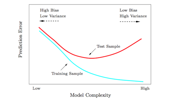
This is the first benefit of regularization: it will likely improve your model’s prediction accuracy on previously unseen data. I use the word “likely” here because you could be operating in the left region of that curve. If that’s the case, you might need to start engineering some features!

What’s the second benefit of regularizing? I previously mentioned that regularization could actually zero our weights for some of your features. This is a nice side effective of regularization—the data helps us with model selection by zeroing out some features! That’s actually the second benefit of regularization: it helps us with model selection by only keeping those features with the strongest effects on our labels. At iHeartRadio we talk about “throwing the kitchen sink” at a modeling problem, knowing that aggressive regularization can limit the effects of spurious predictors. Simpler natural language techniques also take this path, using bag-of-word features, the LASSO, and high values of $\lambda$ to drop all but the most important features.

Ok, let’s regularize

With these benefits in mind, it’s easy to add a regularization term to your objective function. You face two decisions:

1. Your choice of function $R(\mathbf{w})$, and
2. Your choice of regularizing parameter $\lambda$

When addressing the first question, you’ll probably choose between the 1-norm (known as the LASSO, or L1-regularization) and the 2-norm (known as ridge regularization or L2-regularization). These regularizers induce different behaviors in your learned weights. While ridge regularization nudges learned weights downward, the LASSO strongly encourages sparsity in the learned model by favoring $\mathbf{w}_f = 0$ for any feature $f$.

Here’s a brief explanation as to why that’s the case. The objective function $L(w, x)$ above can be restated as a constrained optimization problem of the form:

$$L(\mathbf{w}) = \sum_{i=1}^{N}(y_i - \mathbf{w}^{T}x_i)^{2}$$

subject to the constraint $R(\mathbf{w}) \le \lambda$. Assume that $\mathbf{w}$ and $x_i$ are both in $\mathbb{R}^2$. Since we’ve stuck with the sum of squares error, we can visualize this optimization problem as follows:

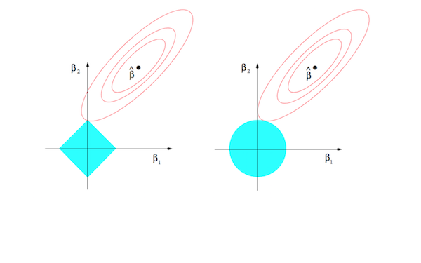
These plots show the space of possible assignments to the parameter estimate $\mathbf{w}$ (let’s assume the component of $\beta$ along each axis is instead a component of $\mathbf{w}$). The blue region in each plot is the constrained space of solutions, while the red contours represent potential values of $\hat{\mathbf{w}}$. We want to find the point inside the constrained space that sits on the contour closest to the solution; for the LASSO region on the left, that point is far more likely to sit along an axis, which would thus yield a sparser solution for $\hat{\mathbf{w}}$.

Returning to the second question, it is common to treat $\lambda$ as a parameter selected via grid search (just make sure to use cross-validation). You could also instead roll with the ElasticNet algorithm, which regularizes your objective function using $R(\mathbf{w}) = \alpha\sum_{i=1}^{M}|\mathbf{w}_i| + (1-\alpha)\sum_{i=1}^{M}\mathbf{w}_{i}^{2}$ while adaptively choosing the best $\alpha$.

Final comments

Some notes on regularizing:

• You should standardize your input dataset so that it is distributed according to $\mathcal{N}(0, 1)$, since solutions to the regularized objective function depend on the scale of your features.
• Both scikit-learn and R have great regularization packages. Check out the scikit-learn docs on GLMs or R’s glmnet.

Julia asked about how one can debug regularization. It is not guaranteed that a regularized model generalizes better than an unregularized model, but I have observed the following in the past:

• If introducing LASSO to your model forces your coefficients to zero, your model is not that great. You might need to reconsider your features.
• Try estimating $\mathbf{w}$ using vanilla regression, then check the 1-norm and 2-norm of $\hat{\mathbf{w}}$. Intuitively-speaking, this unregularized estimate should have a higher norm than its regularized counterpart.

Finally, I aimed for a very straightforward discussion of regularization here. Some interesting follow-up resources:

• EoSL introduces a Bayesian interpretation of regularization — ridge regularization is equivalent to imposing a Gaussian prior on the model parameters — and comments on the relationship to the singular value decomposition (as a feature's singular value under the SVD of $\mathbf{X}$ decreases, its corresponding weight is also downweighted by regularization). Interesting stuff.
• This post used the sum of squares for simplicity, although regularization extends to all sorts of model classes. Section 5.5 of Pattern Recognition and Machine Learning explains how regularization can also mitigate over-fitting when training neural networks, for example.

References

What I actually referenced while writing this post:

1. Hastie, T. et. al. (2009). The Elements of Statistical Learning: Data Mining, Inference, and Prediction. Springer-Verlag.
2. Hastie, T. et. al. (2015). Statistical Learning with Sparsity: The Lasso and Generalizations. Chapman and Hall.
3. Some Wikipedia on various things to refresh my memory.